4.8.2.2. Mean Squared Displacement — MDAnalysis.analysis.msd
- Authors:
Hugo MacDermott-Opeskin
- Year:
2020
- Copyright:
Lesser GNU Public License v2.1+
This module implements the calculation of Mean Squared Displacements (MSDs) by the Einstein relation. MSDs can be used to characterize the speed at which particles move and has its roots in the study of Brownian motion. For a full explanation of the theory behind MSDs and the subsequent calculation of self-diffusivities the reader is directed to [1]. MSDs can be computed from the following expression, known as the Einstein formula:
where \(N\) is the number of equivalent particles the MSD is calculated over, \(r\) are their coordinates and \(d\) the desired dimensionality of the MSD. Note that while the definition of the MSD is universal, there are many practical considerations to computing the MSD that vary between implementations. In this module, we compute a “windowed” MSD, where the MSD is averaged over all possible lag-times \(\tau \le \tau_{max}\), where \(\tau_{max}\) is the length of the trajectory, thereby maximizing the number of samples.
The computation of the MSD in this way can be computationally intensive due to
its \(N^2\) scaling with respect to \(\tau_{max}\). An algorithm to
compute the MSD with \(N log(N)\) scaling based on a Fast Fourier
Transform is known and can be accessed by setting fft=True [Calandri2011]
[Buyl2018]. The FFT-based approach requires that the
tidynamics package is
installed; otherwise the code will raise an ImportError.
Please cite [Calandri2011] [Buyl2018] if you use this module in addition to the normal MDAnalysis citations.
Warning
To correctly compute the MSD using this analysis module, you must supply coordinates in the unwrapped convention, also known as no-jump. That is, when atoms pass the periodic boundary, they must not be wrapped back into the primary simulation cell.
In MDAnalysis you can use the
NoJump
transformation to unwrap coordinates on-the-fly.
A minimal example:
import MDAnalysis as mda
from MDAnalysis.transformations import NoJump

u = mda.Universe(TOP, TRAJ)

# Apply NoJump transformation to unwrap coordinates
u.trajectory.add_transformations(NoJump(u))

# Now the trajectory is unwrapped and MSD can be computed normally:
from MDAnalysis.analysis.msd import EinsteinMSD
MSD = EinsteinMSD(u, select="all", msd_type="xyz")
MSD.run()
This example assumes that the trajectory contains periodic box
dimensions. If no periodic boundary information is present, box
dimensions must be defined before applying NoJump, which can
be accomplished by applying the
set_dimensions
transformation before the
NoJump transformation.
This replaces the need to preprocess trajectories externally.
In GROMACS, for example, this can be done using gmx trjconv with the
-pbc nojump flag.
See also
4.8.2.2.1. Computing an MSD
This example computes a 3D MSD for the movement of 100 particles undergoing a
random walk. Files provided as part of the MDAnalysis test suite are used
(in the variables RANDOM_WALK and
RANDOM_WALK_TOPO)
First load all modules and test data
import MDAnalysis as mda
import MDAnalysis.analysis.msd as msd
from MDAnalysis.tests.datafiles import RANDOM_WALK_TOPO, RANDOM_WALK
Given a universe containing trajectory data we can extract the MSD
analysis by using the class EinsteinMSD
u = mda.Universe(RANDOM_WALK_TOPO, RANDOM_WALK)
MSD = msd.EinsteinMSD(u, select='all', msd_type='xyz', fft=True)
MSD.run()
The MSD can then be accessed as
msd =  MSD.results.timeseries
lagtimes = MSD.results.delta_t_values
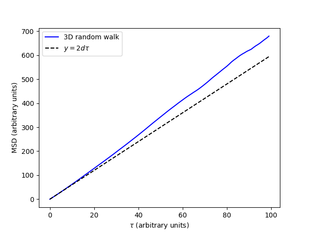
Visual inspection of the MSD is important, so let’s take a look at it with a simple plot.
import matplotlib.pyplot as plt
nframes = MSD.n_frames
fig = plt.figure()
ax = plt.axes()
# plot the actual MSD
ax.plot(lagtimes, msd, lc="black", ls="-", label=r'3D random walk')
exact = lagtimes*6
# plot the exact result
ax.plot(lagtimes, exact, lc="black", ls="--", label=r'$y=2 D\tau$')
plt.show()
This gives us the plot of the MSD with respect to lag-time (\(\tau\)). We can see that the MSD is approximately linear with respect to \(\tau\). This is a numerical example of a known theoretical result that the MSD of a random walk is linear with respect to lag-time, with a slope of \(2d\). In this expression \(d\) is the dimensionality of the MSD. For our 3D MSD, this is 3. For comparison we have plotted the line \(y=6\tau\) to which an ensemble of 3D random walks should converge.
Note that a segment of the MSD is required to be linear to accurately determine self-diffusivity. This linear segment represents the so called “middle” of the MSD plot, where ballistic trajectories at short time-lags are excluded along with poorly averaged data at long time-lags. We can select the “middle” of the MSD by indexing the MSD and the time-lags. Appropriately linear segments of the MSD can be confirmed with a log-log plot as is often reccomended [1] where the “middle” segment can be identified as having a slope of 1.
plt.loglog(lagtimes, msd)
plt.show()
Now that we have identified what segment of our MSD to analyse, let’s compute a self-diffusivity.
4.8.2.2.2. Computing Self-Diffusivity
Self-diffusivity is closely related to the MSD.
From the MSD, self-diffusivities \(D\) with the desired dimensionality \(d\) can be computed by fitting the MSD with respect to the lag-time to a linear model. An example of this is shown below, using the MSD computed in the example above. The segment between \(\tau = 20\) and \(\tau = 60\) is used to demonstrate selection of a MSD segment.
from scipy.stats import linregress
start_time = 20
start_index = int(start_time/timestep)
end_time = 60
linear_model = linregress(lagtimes[start_index:end_index], msd[start_index:end_index])
slope = linear_model.slope
error = linear_model.stderr
# dim_fac is 3 as we computed a 3D msd with 'xyz'
D = slope * 1/(2*MSD.dim_fac)
We have now computed a self-diffusivity!
4.8.2.2.3. Combining Multiple Replicates
It is common practice to combine replicates when calculating MSDs. An example of this is shown below using MSD1 and MSD2.
u1 = mda.Universe(RANDOM_WALK_TOPO, RANDOM_WALK)
MSD1 = msd.EinsteinMSD(u1, select='all', msd_type='xyz', fft=True)
MSD1.run()

u2 = mda.Universe(RANDOM_WALK_TOPO, RANDOM_WALK)
MSD2 = msd.EinsteinMSD(u2, select='all', msd_type='xyz', fft=True)
MSD2.run()

combined_msds = np.concatenate((MSD1.results.msds_by_particle,
                                MSD2.results.msds_by_particle), axis=1)
average_msd = np.mean(combined_msds, axis=1)
The same cannot be achieved by concatenating the replicas in a single run as the jump between the last frame of the first trajectory and frame 0 of the next trajectory will lead to an artificial inflation of the MSD and hence any subsequent diffusion coefficient calculated.
Notes
There are several factors that must be taken into account when setting up and processing trajectories for computation of self-diffusivities. These include specific instructions around simulation settings, using unwrapped trajectories and maintaining a relatively small elapsed time between saved frames. Additionally, corrections for finite size effects are sometimes employed along with various means of estimating errors [2][3] The reader is directed to the following review, which describes many of the common pitfalls [1]. There are other ways to compute self-diffusivity, such as from a Green-Kubo integral. At this point in time, these methods are beyond the scope of this module.
Note also that computation of MSDs is highly memory intensive. If this is
proving a problem, judicious use of the start, stop, step keywords
to control which frames are incorporated may be required.
References
4.8.2.2.4. Classes
- class MDAnalysis.analysis.msd.EinsteinMSD(u, select='all', msd_type='xyz', fft=True, non_linear=False, **kwargs)[source]
Class to calculate Mean Squared Displacement by the Einstein relation.
- Parameters:
u (Universe or AtomGroup) – An MDAnalysis
UniverseorAtomGroup. Note thatUpdatingAtomGroupinstances are not accepted.select (str) – A selection string. Defaults to “all” in which case all atoms are selected.
msd_type ({'xyz', 'xy', 'yz', 'xz', 'x', 'y', 'z'}) – Desired dimensions to be included in the MSD. Defaults to ‘xyz’.
fft (bool) – If
True, uses a fast FFT based algorithm for computation of the MSD. Otherwise, use the simple “windowed” algorithm. The tidynamics package is required for fft=True. Defaults toTrue.non_linear (bool) –
If
True, calculates MSD for trajectory where frames are non-linearly dumped. To use this set fft=False. Defaults toFalse.Added in version 2.10.0.
- results.timeseries
The averaged MSD over all the particles with respect to constant lag-time or unique Δt intervals.
- Type:
- results.msds_by_particle
The MSD of each individual particle with respect to constant lag-time or unique Δt intervals.
for non_linear=False: a 2D array of shape (n_lagtimes, n_atoms)
for non_linear=True: a 2D array of shape (n_delta_t_values, n_atoms)
- Type:
- results.delta_t_values
Array of unique Δt (time differences) at which time-averaged MSD values are computed.
Added in version 2.10.0.
- Type:
- ag
The
AtomGroupresulting from your selection- Type:
AtomGroup
Added in version 2.0.0.
Changed in version 2.10.0: Added ability to calculate MSD from samples that are not linearly spaced with the new non_linear keyword argument.
- classmethod get_supported_backends()
Tuple with backends supported by the core library for a given class. User can pass either one of these values as
backend=...torun()method, or a custom object that hasapplymethod (see documentation forrun()):‘serial’: no parallelization
‘multiprocessing’: parallelization using multiprocessing.Pool
‘dask’: parallelization using dask.delayed.compute(). Requires installation of mdanalysis[dask]
If you want to add your own backend to an existing class, pass a
backends.BackendBasesubclass (see its documentation to learn how to implement it properly), and specifyunsupported_backend=True.- Returns:
names of built-in backends that can be used in
run(backend=...)()- Return type:
Added in version 2.8.0.
- property parallelizable
Boolean mark showing that a given class can be parallelizable with split-apply-combine procedure. Namely, if we can safely distribute
_single_frame()to multiple workers and then combine them with a proper_conclude()call. If set toFalse, no backends except forserialare supported.Note
If you want to check parallelizability of the whole class, without explicitly creating an instance of the class, see
_analysis_algorithm_is_parallelizable. Note that you setting it to other value will break things if the algorithm behind the analysis is not trivially parallelizable.- Returns:
if a given
AnalysisBasesubclass instance is parallelizable with split-apply-combine, or not- Return type:
Added in version 2.8.0.
- run(start: int = None, stop: int = None, step: int = None, frames: Iterable = None, verbose: bool = None, n_workers: int = None, n_parts: int = None, backend: str | BackendBase = None, *, unsupported_backend: bool = False, progressbar_kwargs=None)
Perform the calculation
- Parameters:
start (int, optional) – start frame of analysis
stop (int, optional) – stop frame of analysis
step (int, optional) – number of frames to skip between each analysed frame
frames (array_like, optional) –
array of integers or booleans to slice trajectory;
framescan only be used instead ofstart,stop, andstep. Setting bothframesand at least one ofstart,stop,stepto a non-default value will raise aValueError.Added in version 2.2.0.
verbose (bool, optional) – Turn on verbosity
progressbar_kwargs (dict, optional) – ProgressBar keywords with custom parameters regarding progress bar position, etc; see
MDAnalysis.lib.log.ProgressBarfor full list. Available only forbackend='serial'backend (Union[str, BackendBase], optional) –
By default, performs calculations in a serial fashion. Otherwise, user can choose a backend:
stris matched to a builtin backend (one ofserial,multiprocessinganddask), or aMDAnalysis.analysis.results.BackendBasesubclass.Added in version 2.8.0.
n_workers (int) –
positive integer with number of workers (processes, in case of built-in backends) to split the work between
Added in version 2.8.0.
n_parts (int, optional) –
number of parts to split computations across. Can be more than number of workers.
Added in version 2.8.0.
unsupported_backend (bool, optional) –
if you want to run your custom backend on a parallelizable class that has not been tested by developers, by default False
Added in version 2.8.0.
Changed in version 2.2.0: Added ability to analyze arbitrary frames by passing a list of frame indices in the frames keyword argument.
Changed in version 2.5.0: Add progressbar_kwargs parameter, allowing to modify description, position etc of tqdm progressbars
Changed in version 2.8.0: Introduced
backend,n_workers,n_partsandunsupported_backendkeywords, and refactored the method logic to support parallelizable execution.