12.1.2. Streamplots (3D) — MDAnalysis.visualization.streamlines_3D
- Authors
Tyler Reddy and Matthieu Chavent
- Year
2014
- Copyright
GNU Public License v3
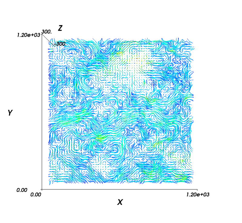
The generate_streamlines_3d() function can generate a 3D flow field from
a MD trajectory, for instance, lipid molecules in a virus capsid. It can make
use of multiple cores to perform the analyis in parallel (using
multiprocessing).
- ᵇChavent2014
Matthieu Chavent, Tyler Reddy, Joseph Goose, Anna Caroline E. Dahl, John E. Stone, Bruno Jobard, and Mark S. P. Sansom. Methodologies for the analysis of instantaneous lipid diffusion in md simulations of large membrane systems. Faraday Discuss., 169:455–475, 2014. doi:10.1039/C3FD00145H.
See also
MDAnalysis.visualization.streamlinesstreamplots in 2D
- MDAnalysis.visualization.streamlines_3D.generate_streamlines_3d(topology_file_path, trajectory_file_path, grid_spacing, MDA_selection, start_frame, end_frame, xmin, xmax, ymin, ymax, zmin, zmax, maximum_delta_magnitude=2.0, num_cores='maximum')[source]
Produce the x, y and z components of a 3D streamplot data set.
- Parameters
topology_file_path (str) – Absolute path to the topology file
trajectory_file_path (str) – Absolute path to the trajectory file. It will normally be desirable to filter the trajectory with a tool such as GROMACS g_filter (see [ᵇChavent2014])
grid_spacing (float) – The spacing between grid lines (angstroms)
MDA_selection (str) – MDAnalysis selection string
start_frame (int) – First frame number to parse
end_frame (int) – Last frame number to parse
xmin (float) – Minimum coordinate boundary for x-axis (angstroms)
xmax (float) – Maximum coordinate boundary for x-axis (angstroms)
ymin (float) – Minimum coordinate boundary for y-axis (angstroms)
ymax (float) – Maximum coordinate boundary for y-axis (angstroms)
maximum_delta_magnitude (float) – Absolute value of the largest displacement tolerated for the centroid of a group of particles ( angstroms). Values above this displacement will not count in the streamplot (treated as excessively large displacements crossing the periodic boundary)
num_cores (int or 'maximum' (optional)) – The number of cores to use. (Default ‘maximum’ uses all available cores)
- Returns
dx_array (array of floats) – An array object containing the displacements in the x direction
dy_array (array of floats) – An array object containing the displacements in the y direction
dz_array (array of floats) – An array object containing the displacements in the z direction
Examples
Generate 3D streamlines and visualize in mayavi:
import numpy as np

import MDAnalysis
import MDAnalysis.visualization.streamlines_3D

import mayavi, mayavi.mlab

# assign coordinate system limits and grid spacing:
x_lower,x_upper = -8.73, 1225.96
y_lower,y_upper = -12.58, 1224.34
z_lower,z_upper = -300, 300
grid_spacing_value = 20

x1, y1, z1 = MDAnalysis.visualization.streamlines_3D.generate_streamlines_3d(
                'testing.gro', 'testing_filtered.xtc',
                 xmin=x_lower, xmax=x_upper,
                 ymin=y_lower, ymax=y_upper,
                 zmin=z_lower, zmax=z_upper,
                 grid_spacing=grid_spacing_value, MDA_selection = 'name PO4',
                 start_frame=2, end_frame=3, num_cores='maximum')

x, y, z = np.mgrid[x_lower:x_upper:x1.shape[0]*1j,
                  y_lower:y_upper:y1.shape[1]*1j,
                  z_lower:z_upper:z1.shape[2]*1j]

# plot with mayavi:
fig = mayavi.mlab.figure(bgcolor=(1.0, 1.0, 1.0), size=(800, 800), fgcolor=(0, 0, 0))
for z_value in np.arange(z_lower, z_upper, grid_spacing_value):
    st = mayavi.mlab.flow(x, y, z, x1, y1, z1, line_width=1,
                          seedtype='plane', integration_direction='both')
    st.streamline_type = 'tube'
    st.tube_filter.radius = 2
    st.seed.widget.origin = np.array([ x_lower,  y_upper,   z_value])
    st.seed.widget.point1 = np.array([ x_upper, y_upper,  z_value])
    st.seed.widget.point2 = np.array([ x_lower, y_lower,  z_value])
    st.seed.widget.resolution = int(x1.shape[0])
    st.seed.widget.enabled = False
mayavi.mlab.axes(extent = [0, 1200, 0, 1200, -300, 300])
fig.scene.z_plus_view()
mayavi.mlab.savefig('test_streamplot_3D.png')
# more compelling examples can be produced for vesicles and other spherical systems